D2l.ai Notes

Disclaimer

These are my personal, raw, notes taken while studying this book.
My aim is to condense the most interesting information on a single page for ease of access, I’ll continue to add more chapters as I continue studying.
The content will sometimes be rephrased by me, sometimes be a copy-paste from the website, sometimes taken from external resources to clarify some concepts I had doubts about.
To delve more into the topics visit their awesome website.

1 - Intro

How can we think of ML?

ML is used when we want to solve a problem for which we cannot precisely codify a solution. For example, creating an ecommerce platform can be codified. But predicting the weather based on location and other data may not! In the example of wake word recognition:

to summarize, rather than code up a wake word recognizer, we code up a program that can learn to recognize wake words

Such learning process consist in “turning some knobs” and determining the optimal set of parameters for our model.

Terminology of data

• Example (or data point, data instance, sample)
• Features (or covariates, inputs)
• Label (or target)
• Inputs are fixed length vectors when each has the same number of features, in this case such number is called dimensionality of data
  • ex: images from the same professional microscope are fixed length, while images gathered from the internet are not
  • modern models can handle varying length of data
• Garbage in Garbage out means that the data needs to be of good quality, cleaned from mistakes This has also implications ethically, where for example an ethnic group is under represented or the data we have is biased

Model

Computational machinery for ingesting data of one type and spitting out predictions of possibly a different type

Objective Functions

We need a measure of how good or bad our models are, these are called objective functions. Traditionally defined such that lower is better, so they are called loss functions.

Some objectives, like squared error, are easy to optimize. Others incur in problems, such as non differentiability, so it is common to use surrogate objectives.

During optimization, we think of the loss as a function of the model’s parameters, and treat the training dataset as a constant.

Also, objective functions need to be evaluated both for training and test data! Doing well in training does not mean that the model will be able to generalize well to unseen data, in such case we talk of overfitting.

Supervised Learning

We are given a dataset containing both features and labels, we need to produce a model which predicts the labels given the input features

We are tipically interested in estimating the conditional probability of a label given the input features.

Regression

Simplest supervised learning task

A good rule of thumb is that any how much? or how many? problem should suggest regression

Usually the loss is a squared error

Classification

Any which one? problem

We want to predict which category (or class) among a discrete set of options

Often our output is in the form of probabilities of belonging to each class.

EX: our classifier needs to distinguish between {cats, dogs}, we get that the probability of an image being cat is 90%, dog 10% → can be interpreted as “the classifier is 90% sure that the image depicts a cat”

• Binary classification : 2 classes
• Multiclass classification : >2 classes
• Hierarchical classification : hierarchically structured classes, ex: animal species

Usually loss is cross-entropy

Tagging

• Multi-label classification : predicting classes which are not mutually exclusive → describe auto-tagging problems (for example when you have to correctly tag a research paper to ease the literature review)

Search

Nowadays ML is widely used for search engines.

Recommender Systems

Recommender systems are another problem setting that is related to search and ranking. The problems are similar insofar as the goal is to display a set of relevant items to the user. The main difference is the emphasis on personalization to specific users in the context of recommender systems.

The customers often provide feedback:

• explicit: star rating and reviews on amazon
• implicit: skipping songs on Spotify

In the simplest formulation, these systems estimate some score, such as the star rating. Then we could retrieve the objects with the highest predicted score to suggest to the user.

Some flaws:

• Censored feedback : the users express their opinion often only when the feel strongly about something, hence the predominance of 5 star or 1 star reviews.
• The result of the actions (ex: buying) of the user are nowadays affected by the recommender system itself.
• feedback loops : an item is sold a lot, hence the algorithm thinks it is good and suggest it, which rises sales even more.

Sequence Learning

The problems before :

• have a fixed number of inputs and produce a fixed number of outputs
• We assumed independence between successive observation → do not hold any memory of predictions

Sequence to sequence: both input and output are variable length sequences

Think of machine translation: you get sentences in a language as input and you have to predict the translation in another language

Some special cases:

• Tagging and parsing: annotating a text sequence with attributes (ex: part-of-speech tagging)
  • here input and output are aligned i.e. they are of the same number and occur in the same order
• Automatic Speech Recognition: input is audio recording, output is the transcription. Here there is no alignment because thousands of samples may correspond to a single word
• Text To Speech: The inverse
• Machine Translation : Here the situation gets more complicated. Inputs and outputs may have different lengths and the order in the sequences may be different

Unsupervised and Self-supervised learning

From Bing:

In machine learning, unsupervised learning is a type of learning where the algorithm learns to identify patterns in the data without any explicit supervision. This means that the algorithm is not given any labeled data, and it must find patterns and structure in the data on its own. Unsupervised learning can be used for tasks such as clustering, anomaly detection, and dimensionality reduction 1.

Self-supervised learning is a specific type of unsupervised learning where the algorithm learns to predict certain properties of the data without any explicit supervision. For example, in image processing, self-supervised learning can be used to predict the rotation angle of an image 2. Self-supervised learning is often used as a pre-training step for supervised learning tasks, where the model is first trained on a large amount of unlabeled data using self-supervised learning, and then fine-tuned on a smaller labeled dataset 23.

In summary, unsupervised learning is a broad category of machine learning algorithms that learn from unlabeled data, while self-supervised learning is a specific type of unsupervised learning that involves predicting certain properties of the data.

In other words:

• SSL is mostly used for pre-training and representation learning. So to bootstrap some model on a later downstream task.
• UL, at least in classical ML, for density estimation and clustering.

Some examples:

• Clustering: ex: you are given a collection of users’ browsing activities, can you group them into users with similar behaviour?
• Subspace estimation (if the dependence is linear → PCA principal component analysis): Can we find a small number of parameters that accurately capture the relevant properties of the data?
• Describe entities and their relation, ex: I have “Rome” − “Italy”, I get “France” = “Paris”
• Causality and probabilistic graphical models: ex: if we have demographic data about house prices, pollution, crime, location, education, and salaries, can we discover how they are related simply based on empirical data?
• Generative models: These models estimate the density of the data, explicitly or implicitly. Early developments with Variational autoencoders, GAN generative adversarial networks, then normalizing flows and diffusion models.

Self Supervised

Leverage some aspect of the un-labelled data to provide supervision

ex:

• predict randomly masked words in a phrase by using the surrounding words
• predict a portion of an image based on the rest of it

Interacting with the environment and Reinforcement Learning

Until now all the learning took place after the algorithm has been disconnected from the environment → Offline Learning

Doing so we do not worry about the complications of interacting with a dynamic environment. But it is limiting, we have something that can do predictions but cannot act… We want agents, not just predictive models

This agent will perform actions that impact the environment, and we need to consider that this impacts also our future observations.

When considering the environment we need to ask ourselves some questions:

• Does the environment remember what we did previously
• Does the environment want to help us? Does it want to beat us? (think of spammers crafting more convincing emails to avoid getting flagged)
• Does the environment have shifting dynamics? (does the future always resemble the past or do the patterns change over time?)

This questions raise the problem of distribution shift, where training and test data are different

Reinforcement learning is a framework for posing problems in which an agent interacts with an environment.

Reinforcement Learning

Reinforcement learning is a framework for posing problems in which an agent interacts with an environment.

It is used in robotics, dialogue systems, or event AI for video games.

Deep reinforcement learning is the application of deep learning to reinforement learning problems → ex : AlphaGo

The general statement is that an agent interacts with an environment over a series of time steps

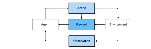
At each time step, the agent receives some observation from the environment and must choose an action that is subsequently transmitted back to the environment via some mechanism (sometimes called an actuator). Finally, the agent receives a reward from the environment.

The behaviour of a reinforcement learning agent is governed by a policy. In short, a policy is just a function that maps from observations of the environment to actions. The goal of reinforcement learning is to produce good policies.

This Framework is very, very general → We can cast supervised learning problems as reinforcement learning ones! The BIG difference is that here we do not know what is the optimal action, we just get a reward and often we do not even know which action led to such reward!!!

The main problems:

• credit assignment: EX: in chess the only reward is at the end of the game, either win or lose, so reinforcement learners must deal with the credit assignment problem (decide which action to blame or to credit for an outcome)
• partial observability : The current observation might not tell you everything about the current state.
• exploit or explore : The algorithm has to decide at any time whether to exploit the best known policy so far, or explore the space of strategies (maybe trading some short term reward)

Categories:

• Markov decision process : the environment is fully observed
• Contextual bandit problem : state does not depend on previous actions
• Multi armed bandit problem : there is no state, just a set of available actions with initial unknown rewards

2 - Preliminaries

1 - Data Manipulation

We’ll use tensors, if 1-dim → array, if 2-dim→matrix

2 - Pre-Processing

Often we get the data in the form of CSV files.

We start by separating columns related to input values from the one with the target value.

Typical problems we need to address:

• NaN values (missing values) : handled with imputation or deletion

3 - Linear Algebra

As said, tensors describe n_th order arrays.

Reduction

Derive some value from the values in the array : ex: the sum of its elements, the mean, etc.

Dot Product

Given two vectors, it is the sum over the products of elements in the same position.

Uses:

• It is often used to compute weighted sums (when the weights are non negative and sum to one, we are doing weighted average)
• After normalizing two vectors to have unit length the dot product express the cosine of the angle between then → (this is a notion of length → cosine similarity)

Matrix - vector products

We can think of multiplication with a matrix A of dimension mxn as a transformation that projects vectors from R of n to R of m → EX: rotations

It is used to compute the output of each of the network layers.

Norms

Informally, the norm of a vector tells us how big it is (magnitude of vector components)

In general we have an l_p norm, best known are the l1 and l2 norms.

In Deep Learning, often we are trying to solve optimization problems: maximizing or minimizing. Often this is expressed in term of distances, which are often expressed as norms

5 - Probability and Statistics

ML is all about uncertainty, we want to predict something which is unknown. Also, sometimes we want to quantify our uncertainty.

Probability

Probability deals with reasoning under uncertainty.

Two Approaches:

• frequentist : probability that applies to repeatable event (ex: coin toss)
• bayesian : more broadly formalizing reasoning under uncertainty
  • assign degrees of belief to non repeatable event (ex : what is the probability of the moon being made of cheese)
  • subjectivity : individuals can start off with different prior beliefs

Statistics

Reason backwards, from the collection of data to doing inferences about the process that generated such data.

Coin tossing example

Formally, the quantity 1/2 is called a probability and here it captures the certainty with which any given toss will come up heads. Probabilities assign scores between 0 and 1 to outcomes of interest, called events. Here the event of interest is heads and we denote the corresponding probability P(heads). A probability of 1 indicates absolute certainty (imagine a trick coin where both sides were heads) and a probability of 0 indicates impossibility (e.g., if both sides were tails).

The frequencies nh/n and nt/n (where nh is the number of heads, nt of tails and n the overall number of tosses) are not probabilities but rather statistics.

Probabilities are theoretical quantities that underlay the data generating process. Here, the probability 1/2 is a property of the coin itself. By contrast, statistics are empirical quantities that are computed as functions of the observed data.

Our interests in probabilistic and statistical quantities are inextricably intertwined. We often design special statistics called estimators that, given a dataset, produce estimates of model parameters like probabilities. Moreover, when those estimators satisfy a nice property called consistency, our estimates will converge to the corresponding probability. In turn, these inferred probabilities tell about the likely statistical properties of data from the same population that we might encounter in the future.

Suppose that we stumbled upon a real coin for which we did not know the true P(heads). To investigate this quantity with statistical methods, we need to (1) collect some data; and (2) design an estimator. Data acquisition here is easy; we can toss the coin many times and record all of the outcomes. Formally, drawing realizations from some underlying random process is called sampling. As you might have guessed, one natural estimator is the fraction between the number of observed heads by the total number of tosses.

In general, for averages of repeated events (like coin tosses), as the number of repetitions grows, our estimates are guaranteed to converge to the true underlying probabilities. The mathematical proof of this phenomenon is called the law of large numbers and the central limit theorem tells us that in many situations, as the sample size n grows, these errors should go down at a rate of (1/√n).

When dealing with randomness, we denote the set of possible outcomes S and call it the sample space or outcome space. Here, each element is a distinct possible outcome. Events are subsets of the sample space.

Recall these axioms of probability:

• The probability of any event A is a non-negative real number, i.e.  
• The probability of the entire sample space is 1, i.e. .
• For any countable sequence of events A1, A2, etc that are mutually exclusive, the probability that any of them happens is equal to the sum of their individual probabilities, i.e.,

Random Variables

Are mappings from an underlying sample space to a set of values.

The occurrence where the random variable X takes value v, denoted by X = v, is an event and P(X = v) denotes its probability

They can be:

• discrete
• continuous

Multiple Random Variables

The probability function that assigns probabilities to combinations (e.g. A=a and B=b) is called the joint probability function.

Conditional probability : P(B=b | A=a) means that we are restricting the attention only to the subset of the sample space associated with A=a and then renormalizing so that all probabilities sum to 1.

Bayes theorem:

This is useful because it allows to reverse the order of conditioning

Also, has a particular interpretation in the setting of Bayesian statistics.

In Bayesian statistics, we think of an observer as possessing some (subjective) prior beliefs about the plausibility of the available hypotheses encoded in the prior P(H), and a likelihood function that says how likely one is to observe any value of the collected evidence for each of the hypotheses in the class P(E | H).

Bayes’ theorem is then interpreted as telling us how to update the initial prior P(H) in light of the available evidence E to produce posterior beliefs P(H|E)=P(E|H)P(H)/P(E). Informally, this can be stated as “posterior equals prior times likelihood, divided by the evidence.

Independence : P(A,B) = P(A|B)P(B) = P(A)P(B)

It is useful when it holds among successive draws of our data from some underlying distribution.

3 - Linear Regression

It stems from few assumptions:

• the relationship between features x and target y is approximately linear (i.e. E[Y|X=x] can be expressed as a weighted sum of features x.
  • this allows for the target value to deviate from the expectation on account of observation noise.
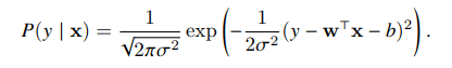
• We can impose that this noise is Gaussian.

An example can be:

w are the weights, while b is the bias (or offset, intercept).

(the bias is always needed, otherwise we are limited to lines that pass through the origin of our system of coordinates)

The learning process will consist of finding w and b that make our model predictions fit to the true values as close as possible.

The dataset of examples will be often referred to as a design matrix, where each row is an example and each column refer to some feature.

This means that predictions can be expressed with a matrix-vector product:

Loss

This function quantifies the distance between the real and predicted values.

The most common loss used for this problems is the squared error.

The 1/2 term does not matter, is there just to be cancelled out when we take the derivative.

The quadratic form of the loss is a double-edged sword:

• avoids large error
• can be susceptible to outliers

To measure the quality of a model on a dataset, we just take the average of the losses over the training set:

Analytic solution

Linear regression is one of the few cases where an analytic solution is possible.

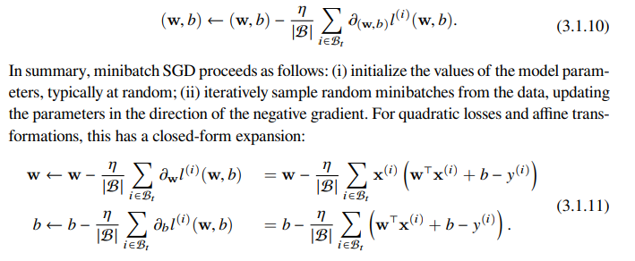
Mini-Batch SGD

This allows to solve models when an analytical solution is not possible or feasible.

It consists in iteratively reduce the error by updating the parameters in the direction by which we lower the loss. → Gradient Descent

How many samples to consider?

• all : most naive applications, drawback is that it is slow to update values of parameters and also we may have some redundancy in our dataset
• one:
  • computational drawback: computers are more efficient (both in energy and time) at matrix-vector multiplication rather than at vector-vector.
  • statistical drawback: some useful layers, like batch normalization, require more than one sample at the time.
• minibatch: you can start from a number between [32,256], the choice depends on memory, accelerators, dataset size, choice of layers.

Mini-Batch Implemented

Learning rate and batch size are user defined → hyperparameters

The solution will correspond to a minimum of the loss

Linear regression is a problem with a global minima, but this is not the usual condition. Finding a good local minima is a challenge usually

Once our model has been trained we can do predictions, called inference.

More about the squared loss and the Gaussian

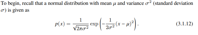
Squared loss can be motivated by assuming that observations arise from noisy measurements, with noise distributed as a gaussian

Then, the likelihood assumes the form:

We can derive the maximum likelihood estimators (to estimate parameters w and b), then take the log and the negative, obtaining the negative log-likelihood, which we need to minimize, it can be expressed as:

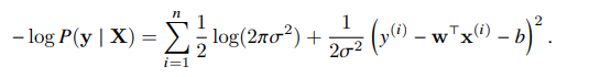
If we consider the sigma constant and disregard the first term, we see that this function reduces to the squared error loss. So, minimizing the squared error is equivalent to maximum likelihood estimation of a linear model under the assumption of additive gaussian noise.

Linear regression can be seen also as a single layer fully connected neural network.

Generalization

Our goal in ML is to discover patterns. This means generalizing well on unseen data.

To do so we must remember that we are training on a limited set of examples, which often cannot cover all the possibilities. This means that doing well on training does not mean we’ll do well on test as well.

Doing well on training but not in test is referred to as overfitting, we’ll try to solve it using regularization techniques.

Training error and generalization error

In standard Supervised Learning we assume that training and test data are drawn independently from identical distributions → IID assumption (this is important!)

• Training error: statistic from the training set →sum
• generalization error: expectation given the underlying distribution of data → integral
  • this cannot calculated, needs to be estimated by applying the model to an independent test set

The model we obtain depends on training set, thus training error is a biased estimate of the true error on the population.

Central question of generalization: When should we expect training error to be close to population error (thus generalization error)

Model complexity:

• simple models and abundant data → training and generalization error tend to be close
• more complex models and fewer examples → training error will go down but generalization gap will grow

Defining model complexity is not straightforward, one idea is to consider the range of values that parameters can take → weight decay is a regularization technique that acts on this.

In general it is also difficult to compare complexities among very different models.

For our result, the only thing we can say is that “low training error alone is not enough to certify low generalization error”. What we do is relying heavily on validation data to certify generalization.

Underfitting or Overfitting

• underfitting : training error and validation error are substantial but there is little gap between them. A low generalization gap suggests we can use a more complex model, the current one may be too simple.
• overfitting : training error is significantly lower than validation.

Dataset size

The fewer the data, the more probable is overfitting.

Sometimes more complex models perform better than simple ones just because of the huge quantity of data at disposal. Otherwise simple models might work better.

Model selection

To do so we need to be wise about the usage of data at our disposal, in the best case we divide it in training, test and validation set.

The distinction between test and validation is muddy.

Sometimes we have not a lot of data, so holdout is not feasible, a possible strategy is Cross-Validation:

Here, the original training data is split into K non-overlapping subsets. Then model training and validation are executed K times, each time training on K −1 subsets and validating on a different subset (the one not used for training in that round). Finally, the training and validation errors are estimated by averaging over the results from the K experiments.

Weight Decay

It’s a regularization technique, recall we can always mitigate overfitting by collecting more training data.

It is also called l2 regularization.

It works by restricting the values that the parameters can take. The idea is that among all functions f, the simplest one is f=0 (returning always zero). Thus we can measure the complexity of a function by measuring the distance between the function parameters and zero. For example, for a function f = wx we might consider some norm of its weight vector.

In order to ensure a small weight vector (i.e. a simple function) is to add its norm as a penalty term in the minimization of the loss.

lambda is the regularization constant.

Often we do not regularize the bias term.

We call this method weight decay because we shrink w to zero.

Why l2?

There are also other norms, like l1, lets discuss:

• l1 : lasso regression → models that concentrate weights on a small set of features by clearing the other weights to zero : gives a method for feature selection
• l2 : ridge regression : places outsize penalty on large components of the weight vector → models that distribute the weight evenly across a larger number of features

4 - Linear NN for Classification

• how to represent the labels? using {1,2,3,} is usually not appropriate because it supposes an ordering among classes which is often not present. A better choice is “one-hot-encoding”
• we need a model with multiple outputs, one per class. In order to use a linear model we need as many affine functions as outputs.

SoftMax

This supposes that we are trying to treat classification as a vector valued regression, however it has several problems. The solution is obtained by using the SoftMax, where we have an exponential function and a normalization. Then, the largest o_i corresponds to the most likely class

Loss function

Usually is the cross-entropy loss

information theory

It deals with the problem of encoding, decoding, transmitting and manipulating information.

Entropy

The central idea in information theory is to quantify the amount of information contained in data.

Given a distribution P, its entropy is

It is the level of surprise experienced by someone who knows the true probability

Surprisal

Compression is linked to prediction. Because, if the next token is easy to predict, then data is easy to compress.

However, if we cannot perfectly predict every event, sometimes we might be surprised. The surprise is greater when we assigned an event a lower probability.

This is the surprisal of observing an event j having assigned it a subjective probability P(j)

The entropy is the expected surprisal when one assigned the correct probabilities that truly match the data-generating process

Cross entropy revisited

The cross-entropy from P to Q, denoted H(P, Q), is the expected surprisal of an observer with subjective probabilities Q upon seeing data that was actually generated according to probabilities P.

In short, we can think of the cross-entropy classification objective in two ways: (i) as maximizing the likelihood of the observed data; and (ii) as minimizing our surprisal (and thus the number of bits) required to communicate the labels.

Image classification dataset

• MNIST : for over a decade was the point of reference for comparing ML algorithms, however now even simple models can achieve very high accuracies, making it unusable to distinguish between models effectively.
• ImageNet : what is used now. However it can be quite big, so for teaching Fashion MNIST might be the best choice, a middle-ground.

Generalization in classification

It turns out that we often can guarantee generalization a-priori: for many models, and for any desired upper bound on the generalization gap ϵ, we can often determine some required number of samples n such that if our training set contains at least n samples, then our empirical error will lie within ϵ of the true error, for any data generating distribution. Unfortunately, it also turns out that while these sorts of guarantees provide a profound set of intellectual building blocks, they are of limited practical utility to the deep learning practitioner. In short, these guarantees suggest that ensuring generalization of deep neural networks a priori requires an absurd number of examples (perhaps trillions or more), even when we find that, on the tasks we care about, deep neural networks typically generalize remarkably well with far fewer examples (thousands). Thus deep learning practitioners often forgo a priori guarantees altogether, instead employing methods on the basis that they have generalized well on similar problems in the past, and certifying generalization post hoc through empirical evaluations.

more theory in the book, quite technical

The most straightforward way to evaluate a model is to consult a test set comprised of previously unseen data. Test set evaluations provide an unbiased estimate of the true error and converge at the desired O(1/√n) rate as the test set grows. We can provide approximate confidence intervals based on exact asymptotic distributions or valid finite sample confidence intervals based on (more conservative) finite sample guarantees. Indeed test set evaluation is the bedrock of modern machine learning research. However, test sets are seldom true test sets (used by multiple researchers again and again). Once the same test set is used to evaluate multiple models, controlling for false discovery can be difficult. This can cause huge problems in theory. In practice, the significance of the problem depends on the size of the holdout sets in question and whether they are merely being used to choose hyperparameters or if they are leaking information more directly. Nevertheless, it is good practice to curate real test sets (or multiple) and to be as conservative as possible about how often they are used. Hoping to provide a more satisfying solution, statistical learning theorists have developed methods for guaranteeing uniform convergence over a model class. If indeed every model’s empirical error converges to its true error simultaneously, then we are free to choose the model that performs best, minimizing the training error, knowing that it too will perform similarly well on the holdout data. Crucially, any of such results must depend on some property of the model class. Vladimir Vapnik and Alexey Chernovenkis introduced the VC dimension, presenting uniform convergence results that hold for all models in a VC class. The training errors for all models in the class are (simultaneously) guaranteed to be close to their true errors, and guaranteed to grow closer at O(1/√ n) rates. Following the revolutionary discovery of VC dimension, numerous alternative complexity measures have been proposed, each facilitating an analogous generalization guarantee

Environment and Distribution shift

Too often, machine learning developers in possession of data rush to develop models without pausing to consider where data comes from in the first place or what we plan to ultimately do with the outputs from our models.

Many failed machine learning deployments can be traced back to this pattern. Sometimes models appear to perform marvellously as measured by test set accuracy but fail catastrophically in deployment when the distribution of data suddenly shifts. More insidiously, sometimes the very deployment of a model can be the catalyst that perturbs the data distribution.

ex : we trained a model to predict who will repay vs. default on a loan, finding that an applicant’s choice of footwear was associated with the risk of default. We might be inclined to thereafter grant loans to all applicants wearing Oxfords and to deny all applicants wearing sneakers. In this case, our ill-considered leap from pattern recognition to decision-making and our failure to critically consider the environment might have disastrous consequences. For starters, as soon as we began making decisions based on footwear, customers would catch on and change their behaviour. Before long, all applicants would be wearing Oxfords, without any coinciding improvement in credit-worthiness.

Types of distribution shift

In one classic setup, we assume that our training data was sampled from some distribution pS(x, y) but that our test data will consist of unlabeled examples drawn from some different distribution pT (x, y). Already, we must confront a sobering reality. Absent any assumptions on how pS and pT relate to each other, learning a robust classifier is impossible.

Fortunately, under some restricted assumptions on the ways our data might change in the future, principled algorithms can detect shift and sometimes even adapt on the fly, improving on the accuracy of the original classifier.

• Covariate shift :

  Here, we assume that while the distribution of inputs may change over time, the labeling function, i.e., the conditional distribution P(y | x) does not change. Statisticians call this covariate shift because the problem arises due to a shift in the distribution of the covariates (features).

  We note that covariate shift is the natural assumption to invoke in settings where we believe that x causes y.

• Label Shift :

  Label shift describes the converse problem. Here, we assume that the label marginal P(y) can change but the class-conditional distribution P(x | y) remains fixed across domains. Label shift is a reasonable assumption to make when we believe that y causes x.

  ex: we may want to predict diagnoses given their symptoms (or other manifestations), even as the relative prevalence of diagnoses are changing over time. Label shift is the appropriate assumption here because diseases cause symptoms.

• Concept shift :

  Arises when the very definitions of labels can change.

  ex: Diagnostic criteria for mental illness, what passes for fashionable, and job titles, are all subject to considerable amounts of concept shift. It turns out that if we navigate around the United States, shifting the source of our data by geography, we will find considerable concept shift regarding the distribution of names for soft drinks.

  US army example

  A similar thing happened to the US Army when they first tried to detect tanks in the forest. They took aerial photographs of the forest without tanks, then drove the tanks into the forest and took another set of pictures. The classifier appeared to work perfectly. Unfortunately, it had merely learned how to distinguish trees with shadows from trees without shadows—the first set of pictures was taken in the early morning, the second set at noon.

• Nonstationary Distributions :

  A much more subtle situation arises when the distribution changes slowly (also known as nonstationary distribution) and the model is not updated adequately

  ex: We build a spam filter. It works well at detecting all spam that we have seen so far. But then the spammers wisen up and craft new messages that look unlike anything we have seen before.

Taxonomy of learning problems

• Batch Learning :

  We have access to training features and labels { (x1, y1), ,(xn, yn) }, which we use to train a model f(x). Later on, we deploy this model to score new data (x, y) drawn from the same distribution. This is the default assumption for any of the problems that we discuss here.

  This is then installed in a customer’s home and is never updated again.

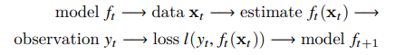
• Online Learning :

  Now imagine that the data (xi, yi) arrives one sample at a time. More specifically, assume that we first observe xi, then we need to come up with an estimate f(xi) and only once we have done this, we observe yi and with it, we receive a reward or incur a loss, given our decision. Many real problems fall into this category. For example, we need to predict tomorrow’s stock price.

  In other words, in online learning, we have the following cycle where we are continuously improving our model given new observations:

  

• Bandits :

  Bandits are a special case of the problem above. While in most learning problems we have a continuously parametrized function f where we want to learn its parameters (e.g., a deep network), in a bandit problem we only have a finite number of actions that we can take.

• Control :

  In many cases the environment remembers what we did. Not necessarily in an adversarial manner but it will just remember and the response will depend on what happened before.

  ex: a coffee boiler controller will observe different temperatures depending on whether it was heating the boiler previously. PID (proportional-integral-derivative) controller algorithms are a popular choice there.

• Reinforcement Learning :

  In the more general case of an environment with memory, we may encounter situations where the environment is trying to cooperate with us , or others where the environment will try to win.

  ex : Chess, Go, Backgammon, or StarCraft

Considering the environment

One key distinction between the different situations above is that the same strategy that might have worked throughout in the case of a stationary environment, might not work throughout when the environment can adapt.

ex : an arbitrage opportunity discovered by a trader is likely to disappear once he starts exploiting it. The speed and manner at which the environment changes determines to a large extent the type of algorithms that we can bring to bear.

Fairness, Accountability and Transparency in ML

It is important to remember that when you deploy machine learning systems you are not merely optimizing a predictive model—you are typically providing a tool that will be used to (partially or fully) automate decisions. These technical systems can impact the lives of individuals subject to the resulting decisions.

Once we contemplate decision-making systems, we must step back and reconsider how we evaluate our technology. Among other consequences of this change of scope, we will find that accuracy is seldom the right measure.

ex : when translating predictions into actions, we will often want to take into account the potential cost sensitivity of erring in various ways. If one way of misclassifying an image could be perceived as a racial sleight of hand, while misclassification to a different category would be harmless, then we might want to adjust our thresholds accordingly, accounting for societal values in designing the decision-making protocol.

We also want to be careful about how prediction systems can lead to feedback loop. ex: consider predictive policing systems, which allocate patrol officers to areas with high forecasted crime.

Often, the various mechanisms by which a model’s predictions become coupled to its training data are unaccounted for in the modelling process. This can lead to what researchers call runaway feedback loops.

5 - MLP Multilayer Perceptron

In this chapter, we will introduce your first truly deep network. The simplest deep networks are called multilayer perceptron and they consist of multiple layers of neurons each fully connected to those in the layer below (from which they receive input) and those above.

Then we will be ready to discuss issues relating to numerical stability and parameter initialization.

When we train such high-capacity models we run the risk of overfitting. Thus, we will revisit regularization and generalization for deep networks.

From linear to non linear

Limitations of linear models

One problem is that linearity implies monotonicity.

Incorporating Hidden Layers

We can stack multiple full connected layers on top of each other. Thus obtain a multi layer perceptron

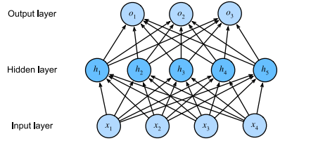
Here there are 4 inputs, 3 outputs and hidden units.

From linear to non linear

The outputs of an hidden layer are called hidden representations.

In order to realize the potential of multilayer architectures, we need one more key ingredient: a nonlinear activation function σ to be applied to each hidden unit following the affine transformation. For instance, a popular choice is the ReLU.

The outputs of activation functions σ(·) are called activations.

Activation Functions

Activation functions decide whether a neuron should be activated or not by calculating the weighted sum and further adding bias with it. They are differentiable operators to transform input signals to outputs, while most of them add non-linearity.

ReLU

The most popular choice, due to both simplicity of implementation and its good performance on a variety of predictive tasks.

The reason for using ReLU is that its derivatives are particularly well behaved: either they vanish or they just let the argument through. This makes optimization better behaved and it mitigated the well-documented problem of vanishing gradients.

Sigmoid

The sigmoid function transforms its inputs, for which values lie in the domain R, to outputs that lie on the interval (0, 1). For that reason, the sigmoid is often called a squashing function.

Tanh

Like the sigmoid function, the tanh (hyperbolic tangent) function also squashes its inputs, transforming them into elements on the interval between -1 and 1.

Forward Propagation, Backward Propagation, and Computational Graphs

The automatic calculation of gradients (automatic differentiation or Autograd) profoundly simplifies the implementation of deep learning algorithms.

Plotting computational graphs helps us visualize the dependencies of operators and variables within the calculation.

Forward propagation (or forward pass) refers to the calculation and storage of intermediate variables (including outputs) for a neural network in order, from the input layer to the output layer.

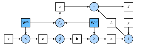
Graph for forward pass:

squares denote variables and circles denote operators. The lower-left corner signifies the input and the upper-right corner is the output. Notice that the directions of the arrows (which illustrate data flow) are primarily rightward and upward

Backpropagation refers to the method of calculating the gradient of neural network parameters. In short, the method traverses the network in reverse order, from the output to the input layer, according to the chain rule from calculus. The algorithm stores any intermediate variables (partial derivatives) required while calculating the gradient with respect to some parameters

When training neural networks, forward and backward propagation depend on each other. In particular, for forward propagation, we traverse the computational graph in the direction of dependencies and compute all the variables on its path. These are then used for backpropagation where the compute order on the graph is reversed.

Forward propagation sequentially calculates and stores intermediate variables within the computational graph defined by the neural network. It proceeds from the input to the output layer. Backpropagation sequentially calculates and stores the gradients of intermediate variables and parameters within the neural network in the reversed order. When training deep learning models, forward propagation and back propagation are interdependent, and training requires significantly more memory than prediction.

Numerical Stability and Initialization

The choice of initialization scheme plays a significant role in neural network learning, and it can be crucial for maintaining numerical stability. Moreover, these choices can be tied up in interesting ways with the choice of the nonlinear activation function.

Vanishing and Exploding gradients

We may be facing parameter updates that are either (i) excessively large, destroying our model (the exploding gradient problem); or (ii) excessively small (the vanishing gradient problem), rendering learning impossible as parameters hardly move on each update.

Vanishing

One frequent culprit causing the vanishing gradient problem is the choice of the activation function σ.

Since early artificial neural networks were inspired by biological neural networks, the idea of neurons that fire either fully or not at all (like biological neurons) seemed appealing.

the sigmoid’s gradient vanishes both when its inputs are large and when they are small. Moreover, when backpropagating through many layers, unless we are in the Goldilocks zone, where the inputs to many of the sigmoids are close to zero, the gradients of the overall product may vanish.

Consequently, ReLUs, which are more stable (but less neurally plausible), have emerged as the default choice for practitioners.

Exploding

The opposite problem, when gradients explode, can be similarly vexing.

Breaking the symmetry

Breaking the symmetry in machine learning refers to the process of introducing differences or distinctions into a model or learning algorithm in order to prevent it from making equivalent or redundant predictions. Symmetry can occur in various forms in machine learning, and breaking it is essential to ensure that the model can learn meaningful and unique representations from the data.

Parameter initialization

One way of addressing—or at least mitigating—the issues raised above is through careful initialization.

Great care in parameter initialization is required to ensure that gradients and parameters remain well controlled. Initialization heuristics are needed to ensure that the initial gradients are neither too large nor too small. Random initialization is key to ensure that symmetry is broken before optimization.

Generalization in Deep Learning

The TL;DR of the present moment is that the theory of deep learning has produced promising lines of attack and scattered fascinating results, but still appears far from a comprehensive account of both (i) why we are able to optimize neural networks and (ii) how models learned by gradient descent manage to generalize so well, even on high-dimensional tasks. However, in practice, (i) is seldom a problem (we can always find parameters that will fit all of our training data) and thus understanding generalization is far the bigger problem. On the other hand, even absent the comfort of a coherent scientific theory, practitioners have developed a large collection of techniques that may help you to produce models that generalize well in practice.

Revisiting overfitting and regularization

According to the “no free lunch” theorem by Wolpert et al. (1995), any learning algorithm generalizes better on data with certain distributions, and worse with other distributions. Thus, given a finite training set, a model relies on certain assumptions: to achieve human-level performance it may be useful to identify inductive biases that reflect how humans think about the world.

With machine learning models encoding inductive biases, our approach to training them typically consists of two phases: (i) fit the training data; and (ii) estimate the generalization error (the true error on the underlying population) by evaluating the model on holdout data. The difference between our fit on the training data and our fit on the test data is called the generalization gap and when the generalization gap is large, we say that our models overfit to the training data.

However deep learning complicates this picture in counterintuitive ways. First, for classification problems, our models are typically expressive enough to perfectly fit every training example, even in datasets consisting of millions.

for many deep learning tasks we are typically choosing among model architectures, all of which can achieve arbitrarily low training loss (and zero training error). Because all models under consideration achieve zero training error, the only avenue for further gains is to reduce overfitting. Even stranger, it is often the case that despite fitting the training data perfectly, we can actually reduce the generalization error further by making the model even more expressive, e.g., adding layers, nodes, or training for a larger number of epochs. Stranger yet, the pattern relating the generalization gap to the complexity of the model (as captured, e.g., in the depth or width of the networks) can be non-monotonic, with greater complexity hurting at first but subsequently helping in a socalled “double-descent” pattern (Nakkiran et al., 2021).

Complicating things even further, while the guarantees provided by classical learning theory can be conservative even for classical models, they appear powerless to explain why it is that deep neural networks generalize in the first place.

Inspiration from NonParametrics

Approaching deep learning for the first time, it is tempting to think of them as parametric models. After all, the models do have millions of parameters. While neural networks, clearly have parameters, in some ways, it can be more fruitful to think of them as behaving like nonparametric models.

So what precisely makes a model nonparametric? While the name covers a diverse set of approaches, one common theme is that nonparametric methods tend to have a level of complexity that grows as the amount of available data grows. Perhaps the simplest example of a nonparametric model is the k-nearest neighbor algorithm.

In a sense, because neural networks are over-parameterized, possessing many more parameters than are needed to fit the training data, they tend to interpolate the training data (fitting it perfectly) and thus behave, in some ways, more like nonparametric models.

Early Stopping

While deep neural networks are capable of fitting arbitrary labels, even when labels are assigned incorrectly or randomly, this ability only emerges over many iterations of training.

A new line of work has revealed that in the setting of label noise, neural networks tend to fit cleanly labeled data first and only subsequently to interpolate the mislabeled data. Moreover, it is been established that this phenomenon translates directly into a guarantee on generalization: whenever a model has fitted the cleanly labeled data but not randomly labeled examples included in the training set, it has in fact generalized.

Together these findings help to motivate early stopping, a classic technique for regularizing deep neural networks.

The most common way to determine the stopping criteria is to monitor validation error throughout training and to cut off training when the validation error has not decreased by more than some small amount ϵ for some number of epochs. This is sometimes called a patience criteria.

Besides the potential to lead to better generalization, in the setting of noisy labels, another benefit of early stopping is the time saved.

Notably, when there is no label noise and datasets are realizable (the classes are truly separable, e.g., distinguishing cats from dogs), early stopping tends not to lead to significant improvements in generalization. On the other hand, when there is label noise, or intrinsic variability in the label (e.g., predicting mortality among patients), early stopping is crucial.

Dropout

Dropout involves injecting noise while computing each internal layer during forward propagation, and it has become a standard technique for training neural networks. The method is called dropout because we literally drop out some neurons during training.

In standard dropout regularization, one zeros out some fraction of the nodes in each layer and then debiases each layer by normalizing by the fraction of nodes that were retained (not dropped out). In other words, with dropout probability p, each intermediate activation h is replaced by a random variable h′ as follows:

7 - CNN Convolutional Neural Networks

Image data is represented as a two-dimensional grid of pixels, be it monochromatic or in color. Accordingly each pixel corresponds to one or multiple numerical values respectively. Preferably, we would leverage our prior knowledge that nearby pixels are typically related to each other, to build efficient models for learning from image data.

In addition to their sample efficiency in achieving accurate models, CNNs tend to be computationally efficient, both because they require fewer parameters than fully connected architectures and because convolutions are easy to parallelize across GPU cores.

From fully connected layers to convolutions

The models that we have discussed so far remain appropriate options when we are dealing with tabular data. However, for high-dimensional perceptual data, such structure-less networks can grow unwieldy. Images exhibit rich structure that can be exploited by humans and machine learning models.

Whatever method we use to recognize objects should not be overly concerned with the precise location of the object in the image. CNNs systematize this idea of spatial invariance, exploiting it to learn useful representations with fewer parameters.

To systematize:

• In the earliest layers, our network should respond similarly to the same patch, regardless of where it appears in the image. This principle is called translation invariance.
• The earliest layers of the network should focus on local regions, without regard for the contents of the image in distant regions. This is the locality principle.
• As we proceed, deeper layers should be able to capture longer-range features of the image, in a way similar to higher level vision in nature.

At page 284, there is a wonderful description of how to go from the MLP to a CNN.

In this section we derived the structure of convolutional neural networks from first principles. While it is unclear whether this is what led to the invention of CNNs, it is satisfying to know that they are the right choice when applying reasonable principles to how image processing and computer vision algorithms should operate, at least at lower levels. In particular, translation invariance in images implies that all patches of an image will be treated in the same manner. Locality means that only a small neighborhood of pixels will be used to compute the corresponding hidden representations.

A second principle that we encountered in our reasoning is how to reduce the number of parameters in a function class without limiting its expressive power.

Adding channels allowed us to bring back some of the complexity that was lost due to the restrictions imposed on the convolutional kernel by locality and translation invariance. Note that channels are quite a natural addition beyond red, green, and blue.

The Cross-Correlation Operation (often improperly called Convolution)

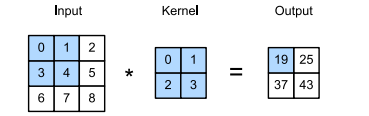
In the two-dimensional cross-correlation operation, we begin with the convolution window positioned at the upper-left corner of the input tensor and slide it across the input tensor, both from left to right and top to bottom. When the convolution window slides to a certain position, the input subtensor contained in that window and the kernel tensor are multiplied elementwise and the resulting tensor is summed up yielding a single scalar value.

the output size is given by the input size nh × nw minus the size of the convolution kernel kh × kw

This is the case since we need enough space to “shift” the convolution kernel across the image. Later we will see how to keep the size unchanged by padding the image with zeros around its boundary so that there is enough space to shift the kernel

A convolutional layer cross-correlates the input and kernel and adds a scalar bias to produce an output. The two parameters of a convolutional layer are the kernel and the scalar bias.

Learning a kernel

Designing a kernel by hand is neat when we know exactly what we are looking for (ex: an edge detector). However, as we look at larger kernels, and consider successive layers of convolutions, it might be impossible to specify precisely what each filter should be doing manually.

Now we see how we can learn the kernel that generated Y from X by looking at the input–output pairs only.

We first construct a convolutional layer and initialize its kernel as a random tensor. Next, in each iteration, we will use the squared error to compare Y with the output of the convolutional layer. We can then calculate the gradient to update the kernel.

Feature Map and Receptive Field

The convolutional layer output is sometimes called a feature map, as it can be regarded as the learned representations (features) in the spatial dimensions (e.g., width and height) to the subsequent layer. In CNNs, for any element x of some layer, its receptive field refers to all the elements (from all the previous layers) that may affect the calculation of x during the forward propagation.

Receptive fields derive their name from neurophysiology.

Final remarks

The core computation required for a convolutional layer is a cross-correlation operation. We saw that a simple nested for-loop is all that is required to compute its value. If we have multiple input and multiple output channels, we are performing a matrix-matrix operation between channels. As can be seen, the computation is straightforward and, most importantly, highly local. This affords significant hardware optimization and many recent results in computer vision are only possible due to that. After all, it means that chip designers can invest into fast computation rather than memory, when it comes to optimizing for convolutions. While this may not lead to optimal designs for other applications, it opens the door to ubiquitous and affordable computer vision.

Padding and stride

We will explore a number of techniques, including padding and strided convolutions, that offer more control over the size of the output. As motivation, note that since kernels generally have width and height greater than 1, after applying many successive convolutions, we tend to wind up with outputs that are considerably smaller than our input. Padding is the most popular tool for handling this issue. In other cases, we may want to reduce the dimensionality drastically, e.g., if we find the original input resolution to be unwieldy. Strided convolutions are a popular technique that can help in these instances.

Padding

One tricky issue when applying convolutional layers is that we tend to lose pixels on the perimeter of our image. The pixels in the corners are hardly used at all.

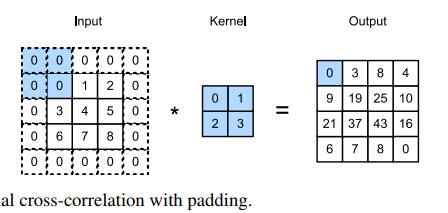
If we add a total of ph rows of padding (roughly half on top and half on bottom) and a total of pw columns of padding (roughly half on the left and half on the right), the output shape will be:

In many cases, we will want to set ph = kh − 1 and pw = kw − 1 to give the input and output the same height and width

CNNs commonly use convolution kernels with odd height and width values, such as 1, 3, 5, or 7. Choosing odd kernel sizes has the benefit that we can preserve the dimensionality while padding with the same number of rows on top and bottom, and the same number of columns on left and right.

Stride

Sometimes, either for computational efficiency or because we wish to downsample, we move our window more than one element at a time, skipping the intermediate locations. This is particularly useful if the convolution kernel is large since it captures a large area of the underlying image. We refer to the number of rows and columns traversed per slide as stride.

In general, when the stride for the height is sh and the stride for the width is sw, the output shape is:

Multiple Input and Multiple Output channels

When we add channels into the mix, our inputs and hidden representations both become three-dimensional tensors. For example, each RGB input image has shape 3 × h × w. We refer to this axis, with a size of 3, as the channel dimension

Multiple Input

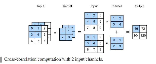
When the input data contains multiple channels, we need to construct a convolution kernel with the same number of input channels as the input data, so that it can perform cross-correlation with the input data. Assuming that the number of channels for the input data is ci, the number of input channels of the convolution kernel also needs to be ci.

However, when ci > 1, we need a kernel that contains a tensor of shape kh × kw for every input channel. Concatenating these ci tensors together yields a convolution kernel of shape ci × kh × kw.

To make sure we really understand what is going on here, we can implement cross-correlation operations with multiple input channels ourselves. Notice that all we are doing is performing a cross-correlation operation per channel and then adding up the results

Multiple Output

Regardless of the number of input channels, so far we always ended up with one output channel. However it turns out to be essential to have multiple channels at each layer.

In the most popular neural network architectures, we actually increase the channel dimension as we go deeper in the neural network, typically downsampling to trade off spatial resolution for greater channel depth. Intuitively, you could think of each channel as responding to a different set of features. The reality is a bit more complicated than this. A naive interpretation would suggest that representations are learned independently per pixel or per channel. Instead, channels are optimized to be jointly useful. This means that rather than mapping a single channel to an edge detector, it may simply mean that some direction in channel space corresponds to detecting edges.

1x1 convolutional layer

At first, a 1×1 convolution, i.e., kh = kw = 1, does not seem to make much sense. After all, a convolution correlates adjacent pixels. A 1 × 1 convolution obviously does not. Nonetheless, they are popular operations that are sometimes included in the designs of complex deep networks.

Because the minimum window is used, the 1 × 1 convolution loses the ability of larger convolutional layers to recognize patterns consisting of interactions among adjacent elements in the height and width dimensions. The only computation of the 1 × 1 convolution occurs on the channel dimension.

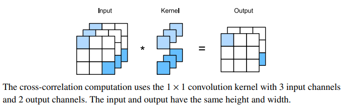
You could think of the 1 × 1 convolutional layer as constituting a fully connected layer applied at every single pixel location to transform the ci corresponding input values into co output values. Because this is still a convolutional layer, the weights are tied across pixel location. Thus the 1×1 convolutional layer requires co×ci weights (plus the bias). Also note that convolutional layers are typically followed by nonlinearities. This ensures that 1 × 1 convolutions cannot simply be folded into other convolutions

Pooling

In many cases our ultimate task asks some global question about the image, e.g., does it contain a cat? Consequently, the units of our final layer should be sensitive to the entire input. By gradually aggregating information, yielding coarser and coarser maps, we accomplish this goal of ultimately learning a global representation, while keeping all of the advantages of convolutional layers at the intermediate layers of processing. The deeper we go in the network, the larger the receptive field (relative to the input) to which each hidden node is sensitive. Reducing spatial resolution accelerates this process, since the convolution kernels cover a larger effective area.

Max and Average Pooling

Like convolutional layers, pooling operators consist of a fixed-shape window that is slid over all regions in the input according to its stride, computing a single output for each location traversed by the fixed-shape window (sometimes known as the pooling window)

the pooling layer contains no parameters (there is no kernel). Instead, pooling operators are deterministic, typically calculating either the maximum or the average value of the elements in the pooling window. These operations are called maximum pooling (max-pooling for short) and average pooling

When processing multi-channel input data, the pooling layer pools each input channel separately, rather than summing the inputs up over channels as in a convolutional layer. This means that the number of output channels for the pooling layer is the same as the number of input channels.

Max-pooling is preferable to average pooling, as it confers some degree of invariance to output. A popular choice is to pick a pooling window size of 2 × 2 to quarter the spatial resolution of output.

LeNet example

Among the first published CNNs to capture wide attention for its performance on computer vision tasks.

At a high level, LeNet (LeNet-5) consists of two parts: (i) a convolutional encoder consisting of two convolutional layers; and (ii) a dense block consisting of three fully connected layers. The basic units in each convolutional block are a convolutional layer, a sigmoid activation function, and a subsequent average pooling operation.

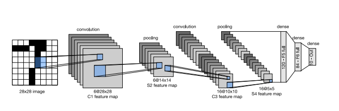
Each convolutional layer uses a 5 × 5 kernel and a sigmoid activation function. These layers map spatially arranged inputs to a number of two-dimensional feature maps, typically increasing the number of channels. The first convolutional layer has 6 output channels, while the second has 16. Each 2 × 2 pooling operation (stride 2) reduces dimensionality by a factor of 4 via spatial downsampling. The convolutional block emits an output with shape given by (batch size, number of channel, height, width).

8 - Modern CNN

Batch Normalization

Training deep neural networks is difficult. Getting them to converge in a reasonable amount of time can be tricky. In this section, we describe batch normalization, a popular and effective technique that consistently accelerates the convergence of deep networks.

Training Deep Networks

When working with data, we often do some preprocessing before training. Choices regarding data preprocessing often make an enormous difference in the final results. For instance, a first step when working with real data might be to standardize our input features to have zero mean µ = 0 and unit variance Σ = 1 across multiple observations.

• Intuitively, this standardization plays nicely with our optimizers since it puts the parameters a priori at a similar scale. As such, it is only natural to ask whether a corresponding normalization step inside a deep network might not be beneficial.
• Second, for a typical MLP or CNN, as we train, the variables in intermediate layers may take values with widely varying magnitudes: both along the layers from input to output, across units in the same layer, and over time due to our updates to the model parameters. The inventors of batch normalization postulated informally that this drift in the distribution of such variables could hamper the convergence of the network. Intuitively, we might conjecture that if one layer has variable activations that are 100 times that of another layer, this might necessitate compensatory adjustments in the learning rates. Adaptive solvers such as AdaGrad or Adam aim to address this from the viewpoint of optimization. The alternative is to prevent the problem from occurring, simply by adaptive normalization.
• Third, deeper networks are complex and tend to be more easily capable of overfitting. This means that regularization becomes more critical.

Batch normalization conveys all three benefits: preprocessing, numerical stability, and regularization.

Batch normalization is applied to individual layers, or optionally, to all of them.

Batch Normalization layers

Batch normalization implementations for fully connected layers and convolutional layers are slightly different. One key difference between batch normalization and other layers is that because batch normalization operates on a full minibatch at a time, we cannot just ignore the batch dimension as we did before when introducing other layer.

• Fully connected layers :

  We can express the computation of a batch-normalization enabled, fully connected layer output h as follows

  Recall that mean and variance are computed on the same minibatch on which the transformation is applied

• Convolutional layers :

  We can apply batch normalization after the convolution and before the nonlinear activation function. The key difference from batch normalization in fully connected layers is that we apply the operation on a per-channel basis across all locations

• Layer Normalization :

  Note that in the context of convolutions the batch normalization is well-defined even for minibatches of size 1: after all, we have all the locations across an image to average. Consequently, mean and variance are well defined, even if it is just within a single observation. This consideration led to introduce the notion of layer normalization. It works just like a batch norm, only that it is applied to one observation at a time. Consequently both the offset and the scaling factor are scalars it does not depend on the minibatch size. It is also independent of whether we are in training or test regime.

  In other words, it is simply a deterministic transformation that standardizes the activations to a given scale. This can be very beneficial in preventing divergence in optimization.

Batch normalization during prediction

As we mentioned earlier, batch normalization typically behaves differently in training mode and prediction mode. First, the noise in the sample mean and the sample variance arising from estimating each on minibatches are no longer desirable once we have trained the model. Second, we might not have the luxury of computing per-batch normalization statistics. For example, we might need to apply our model to make one prediction at a time. Typically, after training, we use the entire dataset to compute stable estimates of the variable statistics and then fix them at prediction time. Consequently, batch normalization behaves differently during training and at test time. Recall that dropout also exhibits this characteristic.

9 - RNN Recurrent Neural Networks

Recurrent neural networks (RNNs) are deep learning models that capture the dynamics of sequences via recurrent connections, which can be thought of as cycles in the network of nodes.

Recurrent neural networks are unrolled across time steps (or sequence steps), with the same underlying parameters applied at each step. While the standard connections are applied synchronously to propagate each layer’s activations to the subsequent layer at the same time step, the recurrent connections are dynamic, passing information across adjacent time steps. RNNs can be thought of as feedforward neural networks where each layer’s parameters (both conventional and recurrent) are shared across time steps.

One key insight paved the way for a revolution in sequence modeling. While the inputs and targets for many fundamental tasks in machine learning cannot easily be represented as fixed length vectors, they can often nevertheless be represented as varying-length sequences of fixed length vectors.

Working with sequences

Up until now, we have focused on models whose inputs consisted of a single feature vector x ∈ Rd. The main change of perspective when developing models capable of processing sequences is that we now focus on inputs that consist of an ordered list of feature vectors.

Some datasets consist of a single massive sequence. Consider, for example, the extremely lon streams of sensor readings that might be available to climate scientists. In such cases, we might create training datasets by randomly sampling subsequences of some predetermined length. More often, our data arrives as a collection of sequences.

Previously, when dealing with individual inputs, we assumed that they were sampled independently from the same underlying distribution P(X). While we still assume that entire sequences (e.g., entire documents or patient trajectories) are sampled independently, we cannot assume that the data arriving at each time step are independent of each other.

For most sequence models, we do not require independence, or even stationarity, of our sequences. Instead, we require only that the sequences themselves are sampled from some fixed underlying distribution over entire sequences.

This flexible approach, allows for such phenomena as (i) documents looking significantly different at the beginning than at the end, or (ii) patient status evolving either towards recovery or towards death over the course of a hospital stay; and (iii) customer taste evolving in predictable ways over course of continued interaction with a recommender system.

Sequence-to-sequence tasks take two forms: (i) aligned: where the input at each time step aligns with a corresponding target (e.g., part of speech tagging); (ii) unaligned: where the input and target do not necessarily exhibit a step-for-step correspondence.

Autoregressive models

Before introducing specialized neural networks designed to handle sequentially structured data, let’s take a look at some actual sequence data and build up some basic intuitions and statistical tools.

One simple strategy for estimating the conditional expectation would be to apply a linear regression model. Such models that regress the value of a signal on the previous values of that same signal are naturally called autoregressive models. There is just one major problem: the number of inputs, xt−1, , x1 varies, depending on t. Namely, the number of inputs increases with the amount of data that we encounter. Thus if we want to treat our historical data as a training set, we are left with the problem that each example has a different number of features.

A few strategies recur frequently. First of all, we might believe that although long sequences xt−1, , x1 are available, it may not be necessary to look back so far in the history when predicting the near future. In this case we might content ourselves to condition on some window of length τ and only use xt−1, , xt−τ observations. The immediate benefit is that now the number of arguments is always the same, at least for t > τ. This allows us to train any linear model or deep network that requires fixed-length vectors as inputs. Second, we might develop models that maintain some summary ht of the past observations and at the same time update ht in addition to the prediction xˆt This leads to models that estimate xt with xˆt = P(xt| ht) and moreover updates of the form ht = g(ht−1, xt−1). Since ht is never observed, these models are also called latent autoregressive models.

To construct training data from historical data, one typically creates examples by sampling windows randomly. In general, we do not expect time to stand still. However, we often assume that while the specific values of xt might change, the dynamics according to which each subsequent observation is generated given the previous observations do not. Statisticians call dynamics that do not change stationary.

Sequence Models

Sometimes, especially when working with language, we wish to estimate the joint probability of an entire sequence. This is a common task when working with sequences composed of discrete tokens, such as words. Generally, these estimated functions are called sequence models and for natural language data, they are called language models.

While language modeling might not look, at first glance, like an autoregressive problem, we can reduce language modeling to autoregressive prediction by decomposing the joint density of a sequence p(xt| x1, , xT ) into the product of conditional densities in a left-to-right fashion by applying the chain rule of probability:

Markov models

Now suppose that we wish to employ the strategy where we condition only on the τ previous time steps, i.e., xt−1, , xt−τ, rather than the entire sequence history xt−1, , x1. Whenever we can throw away the history beyond the precious τ steps without any loss in predictive power, we say that the sequence satisfies a Markov condition, i.e., that the future is conditionally independent of the past, given the recent history. When τ = 1, we say that the data is characterized by a first-order Markov model, and when τ = k, we say that the data is characterized by a k-th order Markov model.

We often find it useful to work with models that proceed as though a Markov condition were satisfied, even when we know that this is only approximately true

With discrete data, a true Markov model simply counts the number of times that each word has occurred in each context, producing the relative frequency estimate of P(xt | xt−1).

Prediction

Consider, what if we only observed sequence data up until time step 604 (n_train + tau) but wished to make predictions several steps into the future.

We can address this problem by plugging in our earlier predictions as inputs to our model for making subsequent predictions, projecting forward, one step at a time, until reaching the desired time step:

Generally, for an observed sequence x1, , xt, its predicted output xˆt+k at time step t+ k is called the k-step-ahead prediction

Why did the algorithm perform so much worse when predicting further into the future? Ultimately, this owes to the fact that errors build up. Let’s say that after step 1 we have some error ϵ1 = ϵ¯. Now the input for step 2 is perturbed by ϵ1, hence we suffer some error in the order of ϵ2 = ϵ¯+ cϵ1 for some constant c, and so on. The predictions can diverge rapidly from the true observations. You may already be familiar with this common phenomenon. For instance, weather forecasts for the next 24 hours tend to be pretty accurate but beyond that, accuracy declines rapidly.

Converting Raw text into sequence data

Throughout this book, we will often work with text data represented as sequences of words, characters, or word-pieces. To get going, we will need some basic tools for converting raw text into sequences of the appropriate form. Typical preprocessing pipelines execute the following steps:

• Load text as strings into memory.
• Split the strings into tokens.
• Build a vocabulary dictionary to associate each vocabulary element with a numerical index.
• Convert the text into sequences of numerical indices.

Tokenization

Tokens are the atomic (indivisible) units of text. Each time step corresponds to 1 token, but what precisely constitutes a token is a design choice.

For example, we could represent the sentence “Baby needs a new pair of shoes” as a sequence of 7 words, where the set of all words comprise a large vocabulary (typically tens or hundreds of thousands of words). Or we would represent the same sentence as a much longer sequence of 30 characters, using a much smaller vocabulary.

Vocabulary

These tokens are still strings. However, the inputs to our models must ultimately consist of numerical inputs. Next, we introduce a class for constructing vocabularies, i.e., objects that associate each distinct token value with a unique index. First, we determine the set of unique tokens in our training corpus. We then assign a numerical index to each unique token.

Exploratory language statistics

Articles like “the” and “a”, pronouns like “i” and “my”, and prepositions like “of”, “to”, and “in” occur often because they serve common syntactic roles. Such words that are at once common but particularly descriptive are often called stop words and, in previous generations of text classifiers based on bag-of-words representations, they were most often filtered out. However, they carry meaning and it is not necessary to filter them out when working with modern RNN- and Transformer based neural models.

You will notice that word frequency decays quickly. The 10th most frequent word is less than 1/5 as common as the most popular. Word frequency tends to follow a power law distribution (specifically the Zipfian) as we go down the ranks

Let’s visualize the token frequency among these three models: unigrams, bigrams, and trigrams

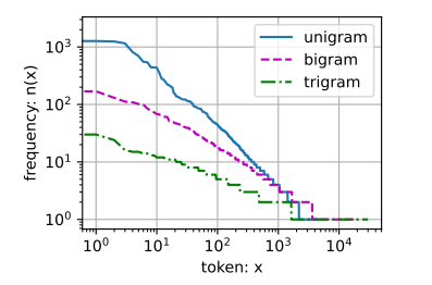
This figure is quite exciting. First, beyond unigram words, sequences of words also appear to be following Zipf law, albeit with a smaller exponent α in, depending on the sequence length. Second, the number of distinct n-grams is not that large. This gives us hope that there is quite a lot of structure in language. Third, many n-grams occur very rarely. This makes certain methods unsuitable for language modeling and motivates the use of deep learning models.

Language models

The goal of language models is to estimate the joint probability of the whole sequence:

Language models are incredibly useful. For instance, an ideal language model would be able to generate natural text just on its own, simply by drawing one token at a time.

We are still very far from designing such a system, since it would need to understand the text rather than just generate grammatically sensible content. Nonetheless, language models are of great service even in their limited form. For instance, the phrases “to recognize speech” and “to wreck a nice beach” sound very similar. This can cause ambiguity in speech recognition, which is easily resolved through a language model that rejects the second translation as outlandish.

Learning language models

Markov models and n-grams

. A distribution over sequences satisfies the Markov property of first order if P( xt+1 | xt, , x1) = P(xt+1 | xt). Higher orders correspond to longer dependencies. This leads to a number of approximations that we could apply to model a sequence:

The probability formulae that involve one, two, and three variables are typically referred to as unigram, bigram, and trigram models, respectively. In order to compute the language model,

we need to calculate the probability of words and the conditional probability of a word given the previous few words. Note that such probabilities are language model parameters.

Word Frequency

Here, we assume that the training dataset is a large text corpus, such as all Wikipedia.

The probability of words can be calculated from the relative word frequency of a given word in the training dataset.

A slightly less accurate approach would be to count all occurrences of the word “deep” and divide it by the total number of words in the corpus. This works fairly well, particularly for frequent words.

Moving on, we could attempt to estimate

where n(x) and n(x, x′) are the number of occurrences of singletons and consecutive word pairs, respectively. Unfortunately, estimating the probability of a word pair is somewhat more difficult, since the occurrences of “deep learning” are a lot less frequent.

Unless we provide some solution to assign such word combinations nonzero count, we will not be able to use them in a language model. If the dataset is small or if the words are very rare, we might not find even a single one of them.

A common strategy is to perform some form of Laplace smoothing. The solution is to add a small constant to all counts

Unfortunately, models like this get unwieldy rather quickly for the following reasons. First, many n-grams occur very rarely, making Laplace smoothing rather unsuitable for language modeling. Second, we need to store all counts. Third, this entirely ignores the meaning of the words

hence a model that simply counts the frequency of previously seen word sequences is bound to perform poorly there. Therefore, we focus on using neural networks for language modeling in the rest of the chapter

Perplexity

Next, let’s discuss about how to measure the language model quality, which will be used to evaluate our models in the subsequent sections. One way is to check how surprising the text is.

We might measure the quality of the model by computing the likelihood of the sequence. Unfortunately this is a number that is hard to understand and difficult to compare. After all, shorter sequences are much more likely to occur than the longer ones, hence evaluating the model on Tolstoy’s magnum opus War and Peace will inevitably produce a much smaller likelihood than, say, on Saint-Exupery’s novella The Little Prince. What is missing is the equivalent of an average.

Information theory comes handy here. We have defined entropy, surprisal, and cross-entropy when we introduced the SoftMax regression (Section 4.1.3). If we want to compress text, we can ask about predicting the next token given the current set of tokens. A better language model should allow us to predict the next token more accurately. Thus, it should allow us to spend fewer bits in compressing the sequence. So we can measure it by the cross-entropy loss averaged over all the n tokens of a sequence.

For historical reasons, scientists in natural language processing prefer to use a quantity called perplexity. In a nutshell, it is the exponential of the cross entropy loss.

Perplexity can be best understood as the geometric mean of the number of real choices that we have when deciding which token to pick next.

Recurrent neural networks

Recurrent neural networks (RNNs) are neural networks with hidden states.

From the relationship between hidden layer outputs Ht and Ht−1 of adjacent time steps, we know that these variables captured and retained the sequence’s historical information up to their current time step, just like the state or memory of the neural network’s current time step. Therefore, such a hidden layer output is called a hidden state. Since the hidden state uses the same definition of the previous time step in the current time step, the computation of is recurrent. Hence, as we said, neural networks with hidden states based on recurrent computation are named recurrent neural networks. Layers that perform the computation of (9.4.5) in RNNs are called recurrent layers.

Parameters of the RNN include the weights Wxh ∈ Rd×h,Whh ∈ Rh×h, and the bias bh ∈R1×h of the hidden layer, together with the weights Whq ∈ Rh×qand the bias bq ∈ R1×q of the output layer. It is worth mentioning that even at different time steps, RNNs always use these model parameters. Therefore, the parameterization cost of an RNN does not grow as the number of time steps increases

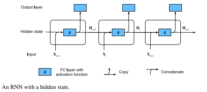
One-Hot Encoding

Recall that each token is represented by a numerical index indicating the position in the vocabulary of the corresponding word/character/word-piece

This works when we are dealing with numerical inputs like price or temperature, where any two values sufficiently close together should be treated similarly. But this does not quite make sense. The 45th and 46th words in our vocabulary happen to be “their” and “said”, whose meanings are not remotely similar.

When dealing with such categorical data, the most common strategy is to represent each item by a one-hot encoding. A one-hot encoding is a vector whose length is given by the size of the vocabulary N, where all entries are set to 0, except for the entry corresponding to our token, which is set to 1.

Gradient Clipping

While you are already used to thinking of neural networks as “deep” in the sense that many layers separate the input and output even within a single time step, the length of the sequence introduces a new notion of depth.

Taking the backwards view, in each iteration, we backpropagate gradients through time, resulting in a chain of matrix-products with length O(T). This can result in numerical instability, causing the gradients to either explode or vanish depending on the properties of the weight matrices. Dealing with vanishing and exploding gradients is a fundamental problem when designing RNN.

One inelegant but ubiquitous solution is to simply clip the gradients forcing the resulting “clipped” gradients to take smaller values.

Backpropagation through time

Applying backpropagation in RNNs is called backpropagation through time. This procedure requires us to expand (or unroll) the computational graph of an RNN one time step at a time. The unrolled RNN is essentially a feedforward neural network with the special property that the same parameters are repeated throughout the unrolled network, appearing at each time step. Then, just as in any feedforward neural network, we can apply the chain rule, backpropagating gradients through the unrolled net.

Complications arise because sequences can be rather long. It is not unusual to work with text sequences consisting of over a thousand tokens. Note that this poses problems both from a computational (too much memory) and optimization (numerical instability) standpoint.

10 - Modern RNN

In this chapter, we introduce the key ideas behind the most successful RNN architectures for sequence, which stem from two papers published in 1997. The first paper, Long-Short Term Memory, introduces the memory cell, a unit of computation that replaces traditional nodes in the hidden layer of a network. With these memory cells, networks are able to overcome difficulties with training encountered by earlier recurrent networks. Intuitively, the memory cell avoids the vanishing gradient problem by keeping values in each memory cell’s internal state cascading along a recurrent edge with weight 1 across many successive time steps. A set of multiplicative gates help the network to determine both which inputs to allow into the memory state, and when the content of the memory state should influence the model’s output.

The second paper, Bidirectional Recurrent Neural Networks (Schuster and Paliwal, 1997), introduces an architecture in which information from both the future (subsequent time steps) and the past (preceding time steps) are used to determine the output at any point in the sequence.

The first sections in this chapter will explain the LSTM architecture, a lighter-weight version called the gated recurrent unit (GRU), the key ideas behind bidirectional RNNs and a brief explanation of how RNN layers are stacked together to form deep RNNs. Subsequently, we will explore the application of RNNs in sequence-to-sequence tasks, introducing machine translation along with key ideas such as encoder-decoder architectures and beam search.

LSTM long short term memory

Shortly after the first Elman-style RNNs were trained using backpropagation (Elman, 1990), the problems of learning long-term dependencies (owing to vanishing and exploding gradients) became salient.

While gradient clipping helps with exploding gradients, handling vanishing gradients appears to require a more elaborate solution. One of the first and most successful techniques for addressing vanishing gradients came in the form of the long short-term memory (LSTM) model due to Hochreiter and Schmidhuber (1997). LSTMs resemble standard recurrent neural networks but here each ordinary recurrent node is replaced by a memory cell. Each memory cell contains an internal state, i.e., a node with a self-connected recurrent edge of fixed weight 1, ensuring that the gradient can pass across many time steps without vanishing or exploding

The term “long short-term memory” comes from the following intuition. Simple recurrent neural networks have long-term memory in the form of weights. The weights change slowly during training, encoding general knowledge about the data. They also have short-term memory in the form of ephemeral activations, which pass from each node to successive nodes. The LSTM model introduces an intermediate type of storage via the memory cell. A memory cell is a composite unit, built from simpler nodes in a specific connectivity pattern, with the novel inclusion of multiplicative nodes.

Gated memory cell

Each memory cell is equipped with an internal state and a number of multiplicative gates that determine whether (i) a given input should impact the internal state (the input gate), (ii) the internal state should be flushed to 0 (the forget gate), and (iii) the internal state of a given neuron should be allowed to impact the cell’s output (the output gate).

Gated Hidden states

The key distinction between vanilla RNNs and LSTMs is that the latter support gating of the hidden state. This means that we have dedicated mechanisms for when a hidden state should be updated and also when it should be reset.

Input Gate, Forget Gate, and Output Gate

The data feeding into the LSTM gates are the input at the current time step and the hidden state of the previous time step. Three fully connected layers with sigmoid activation functions compute the values of the input, forget, and output gates. As a result of the sigmoid activation, all values of the three gates are in the range of (0, 1). Additionally, we require an input node, typically computed with a tanh activation function. Intuitively, the input gate determines how much of the input node’s value should be added to the current memory cell internal state. The forget gate determines whether to keep the current value of the memory or flush it. And the output gate determines whether the memory cell should influence the output at the current time step.

Input Node

Memory Cell Internal State

Hidden state

Gated Recurrent Units (GRU)

As RNNs and particularly the LSTM architecture rapidly gained popularity during the 2010s, a number of papers began to experiment with simplified architectures in hopes of retaining the key idea of incorporating an internal state and multiplicative gating mechanisms but with the aim of speeding up computation. The gated recurrent unit (GRU) (Cho et al., 2014) offered a streamlined version of the LSTM memory cell that often achieves comparable performance but with the advantage of being faster to compute.

Reset Gate and Update Gate

Here, the LSTM’s three gates are replaced by two: the reset gate and the update gate. As with LSTMs, these gates are given sigmoid activations, forcing their values to lie in the interval (0,1).

Intuitively, the reset gate controls how much of the previous state we might still want to remember. Likewise, an update gate would allow us to control how much of the new state is just a copy of the old state.

Deep Recurrent Neural Network

Up until now, we have focused on defining networks consisting of a sequence input, a single hidden RNN layer, and an output layer. Despite having just one hidden layer between the input at any time step and the corresponding output, there is a sense in which these networks are deep. Inputs from the first time step can influence the outputs at the final time step T (often 100s or 1000s of steps later). These inputs pass through T applications of the recurrent layer before reaching the final output. However, we often also wish to retain the ability to express complex relationships between the inputs at a given time step and the outputs at that same time step. Thus we often construct RNNs that are deep not only in the time direction but also in the input-to-output direction. This is precisely the notion of depth that we have already encountered in our development of MLPs and deep CNNs. The standard method for building this sort of deep RNN is strikingly simple: we stack the RNNs on top of each other. Given a sequence of length T, the first RNN produces a sequence of outputs, also of length T.

Bidirectional Recurrent Neural Network

So far, our working example of a sequence learning task has been language modeling, where we aim to predict the next token given all previous tokens in a sequence. In this scenario, we wish only to condition upon the leftward context, and thus the unidirectional chaining of a standard RNN seems appropriate. However, there are many other sequence learning tasks contexts where it is perfectly fine to condition the prediction at every time step on both the leftward and the rightward context.

Another common task—often useful as a pretraining exercise prior to fine-tuning a model on an actual task of interest—is to mask out random tokens in a text document and then to train a sequence model to predict the values of the missing tokens. Note that depending on what comes after the blank, the likely value of the missing token changes dramatically:

• I am __
• I am __ hungry
• I am __ hungry, and I can eat half a pig

In the first sentence “happy” seems to be a likely candidate. The words “not” and “very” seem plausible in the second sentence, but “not” seems incompatible with the third sentences. Fortunately, a simple technique transforms any unidirectional RNN into a bidirectional RNN (Schuster and Paliwal, 1997). We simply implement two unidirectional RNN layers chained together in opposite directions and acting on the same input

Machine Translation

Among the major breakthroughs that prompted widespread interest in modern RNNs was a major advance in the applied field of statistical machine translation. Here, the model is presented with a sentence in one language and must predict the corresponding sentence in another language.

Many problems have this flavor of mapping between two such “unaligned” sequences. Examples include mapping from dialog prompts to replies or from questions to answers. Broadly, such problems are called sequence-to-sequence (seq2seq).

The encoder-decoder architecture

In general seq2seq problems like machine translation (Section 10.5), inputs and outputs are of varying lengths that are unaligned. The standard approach to handling this sort of data is to design an encoder-decoder architecture (Fig. 10.6.1) consisting of two major components: an encoder that takes a variable-length sequence as input, and a decoder that acts as a conditional language model, taking in the encoded input and the leftwards context of the target sequence and predicting the subsequent token in the target sequence

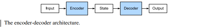
Encoder-Decoder Seq2Seq for Machine Translation

In so-called seq2seq problems like machine translation, where inputs and outputs both consist of variable-length unaligned sequences, we generally rely on encoder-decoder architectures. In this section, we will demonstrate the application of an encoder-decoder architecture, where both the encoder and decoder are implemented as RNNs, to the task of machine translation. Here, the encoder RNN will take a variable-length sequence as input and transform it into a fixed-shape hidden state. Later, in Chapter 11, we will introduce attention mechanisms, which allow us to access encoded inputs without having to compress the entire input into a single fixed-length representation. Then to generate the output sequence, one token at a time, the decoder model, consisting of a separate RNN, will predict each successive target token given both the input sequence and the preceding tokens in the output. During training, the decoder will typically be conditioned upon the preceding tokens in the official “ground-truth” label. However, at test time, we will want to condition each output of the decoder on the tokens already predicted. Note that if we ignore the encoder, the decoder in a seq2seq architecture behaves just like a normal language model.

Teacher Forcing

While running the encoder on the input sequence is relatively straightforward, how to handle the input and output of the decoder requires more care. The most common approach is sometimes called teacher forcing. Here, the original target sequence (token labels) is fed into the decoder as input.

Beam Search

In Section 10.7, we introduced the encoder-decoder architecture, and the standard techniques for training them end-to-end. However, when it came to test-time prediction, we mentioned only the greedy strategy, where we select at each time step the token given the highest predicted probability of coming next, until, at some time step, we find that we have predicted the special end-of-sequence token. In this section, we will begin by formalizing this greedy search strategy and identifying some problems that practitioners tend to run into. Subsequently, we compare this strategy with two alternatives: exhaustive search (illustrative but not practical) and beam search (the standard method in practice).

14 - Computer Vision

In Chapter 7 and Chapter 8, we studied various convolutional neural networks that are commonly used in computer vision, and applied them to simple image classification tasks. At the beginning of this chapter, we will describe two methods that may improve model generalization, namely image augmentation and fine-tuning, and apply them to image classification. Since deep neural networks can effectively represent images in multiple levels, such layerwise representations have been successfully used in various computer vision tasks such as object detection, semantic segmentation, and style transfer.